
Lecture Magdeburg 2001 - Overview
Aus Transnational-Renewables
| Lecture Magdeburg [2001,en], Vortrag Lübeck [2006,de], Lecture Barcelona [2008,en], Vortrag EWEA 2000 [2000,en] |
| Vorstellung regenerativer Energien: Biomasse, Windenergie, Fallwindkraftwerke, Geothermie, Wasserkraft, Solarenergie |
Global Renewable Energy Potential
- Approaches to its Use, held in Magdeburg, Germany on September 2001
|
In my talk I would like to introduce you to the worldwide potentials of renewable electricity production. The techniques we will discuss are electricity production via photovoltaics, solar thermal power plants, hydropower, biomass, hot dry rock geothermal power plants, energy towers and finally we will focus on wind energy. For each of these options of power generation I am going to point out the characteristics with regard to their specific temporal behaviour and the costs to be expected.
We will see that the temporal behaviour significantly changes with the size and the selection of the catchment area used for the power generation. We will also touch on the topics of backup and storage needs and the subject of grid capacities. After this I consider wind energy as major source of power production. And last but not least we will reflect on a possible combination of climate protection and development aid. |
|
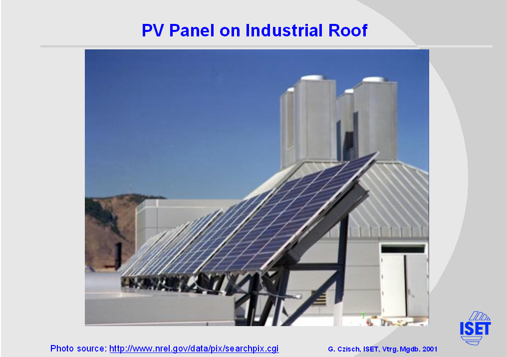
Let‘s start with photovoltaic electricity production. |
|
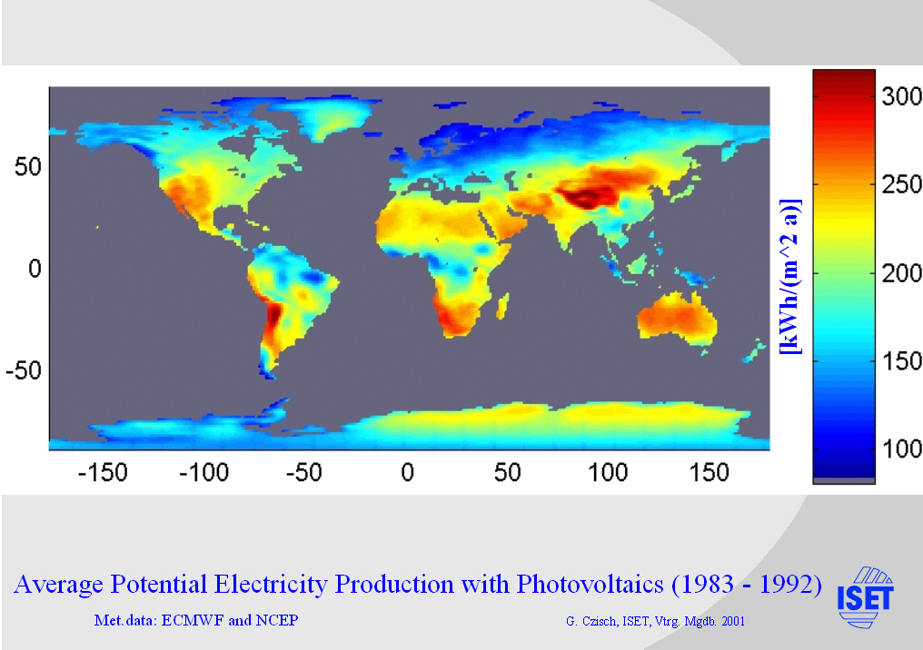
Here you can see the potential production of PV panels mounted in such a way that the orientation of the surface is parallel to the latitude and has a fixed slope equivalent to the latitude towards the sun. The output is calculated from data of the European Centre for Medium Range Weather Forecast (ECMWF) and additional data from the National Centre for Environmental Prediction (NCEP). (The panels are considered to have an efficiency of 14 % at peak radiation and standard temperature reduced to approx. 13 % efficiency due to system losses.)
The best conditions are found in arid zones of high mountainous regions. Here the potential production is more than twice as high as we can expect in middle European countries. In Poland the production of a photovoltaic system will lie in the range of 130 kWh / (m² a) or approx. 900 Full Load Hours (FLH). |

|
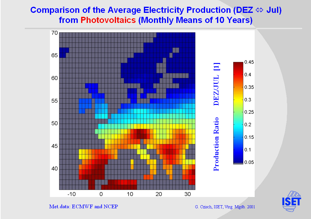
The seasonal variation of power production from PV panels is significantly lower at lower latitudes. On this slide you can see for example the ratio between the average electricity production in December and July. In the southern Sahara we find that the production only changes very slightly over the months while in Europe the winter production is only a small fraction of the summer production. |
|
Here the European conditions are shown. The seasonal variation of power production from PV panels for example in Northern Germany as well as in Northern Poland in December reaches only 10 % of the production in July. In Southern Europe the seasonal fluctuations are significantly lower. |
|
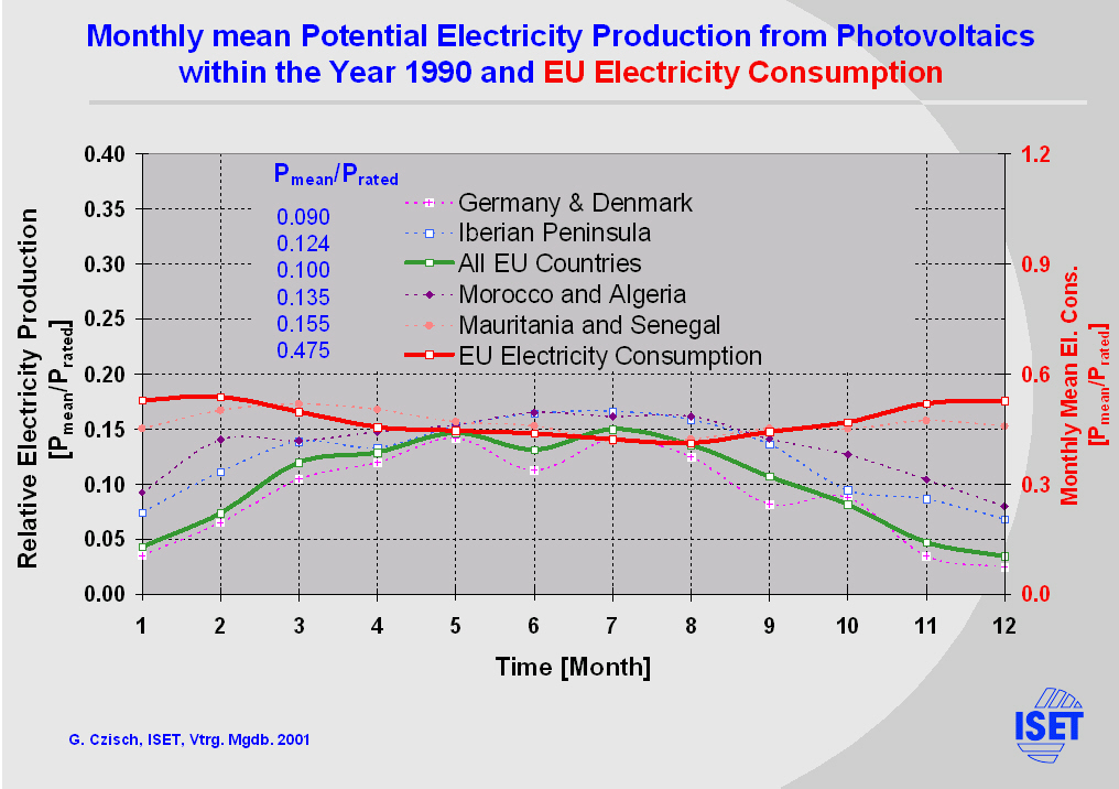
The monthly variation of PV power production can be studied in more detail comparing the different graphs on this slide. They show monthly averages for selected regions contrasted with the electricity consumption of the member states of the EU.
In this example only the production of Mauritania and Senegal in the Southern Sahara show a monthly variation similar to the mentioned electricity consumption. Within all the other regions the behaviour more or less shows an anticyclical pattern compared to the demand. |
|
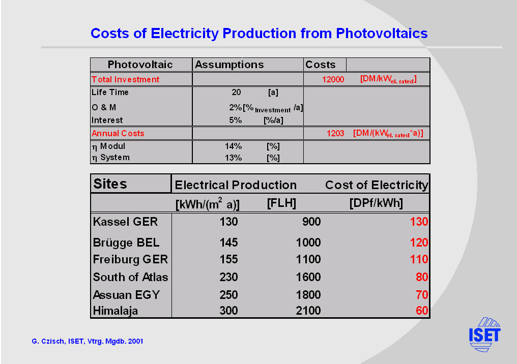
With the underlying economic assumptions shown in the upper table the costs of PV electricity production at some selected sites are calculated and the results are listed in the lower table.
The costs of PV electricity production are relatively high, so that at the today's investment it seems to be an option for rural areas with high potential and without grid connection where it competes with other sometimes even more expensive techniques. |
|
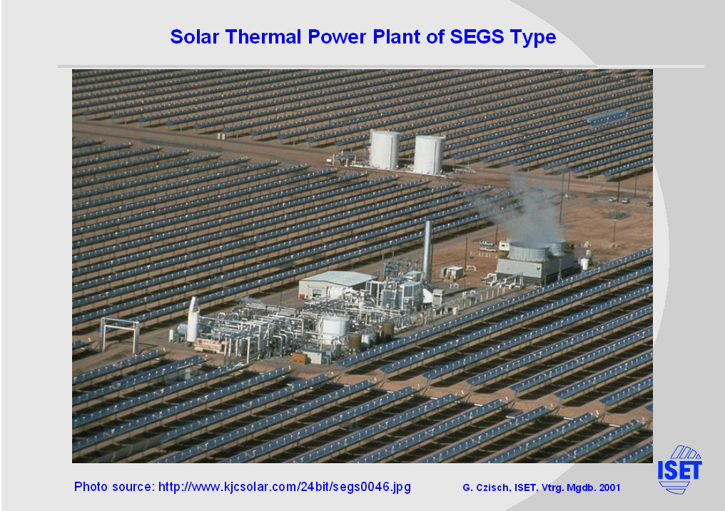
Here you see a view of a solar thermal power plant which leads us to the potentials of this kind of electricity production. The direct solar radiation is concentrated in parabolic troughs to heat up a fluid that is used to power a conventional thermal power plant. Dependent on the design of the power plant the heat is used with an efficiency between approx. 32 and 38 % to produce electricity. |
|
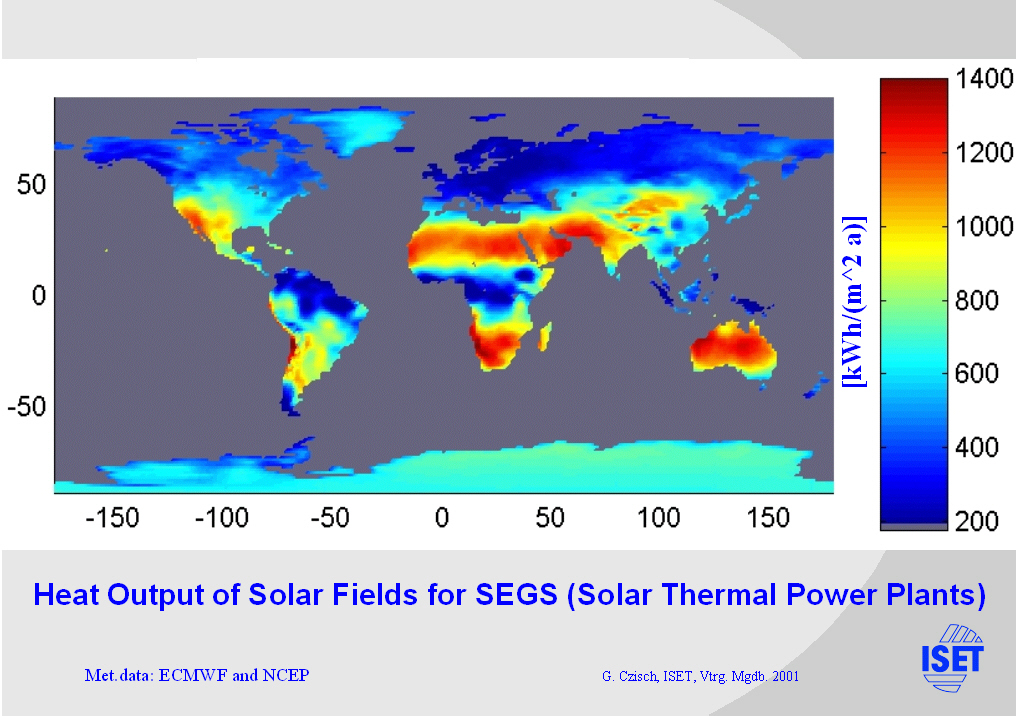
Here the potential heat production of the solar field of a SEGS power plant is shown. Very good conditions are found in the Sahara where the potential electricity production is more than 500 times the electricity consumption of the EU member states. |
|
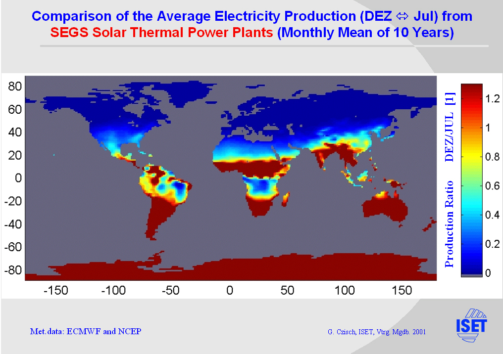
The seasonal variation of power production from SEGS power plants is significantly lower at lower latitudes.
On this slide you can see for example the ratio between the average electricity production in December and July. As it is the case for the PV electricity production, in the southern Sahara we find that the production only changes slightly over the months while the variations increase considerably going to higher longitudes. |

|
The monthly variation of power production from SEGS power plants can be studied in more detail comparing the different graphs on this slide. They show monthly averages for selected regions contrasted with the electricity consumption of the member states of the EU. |
|
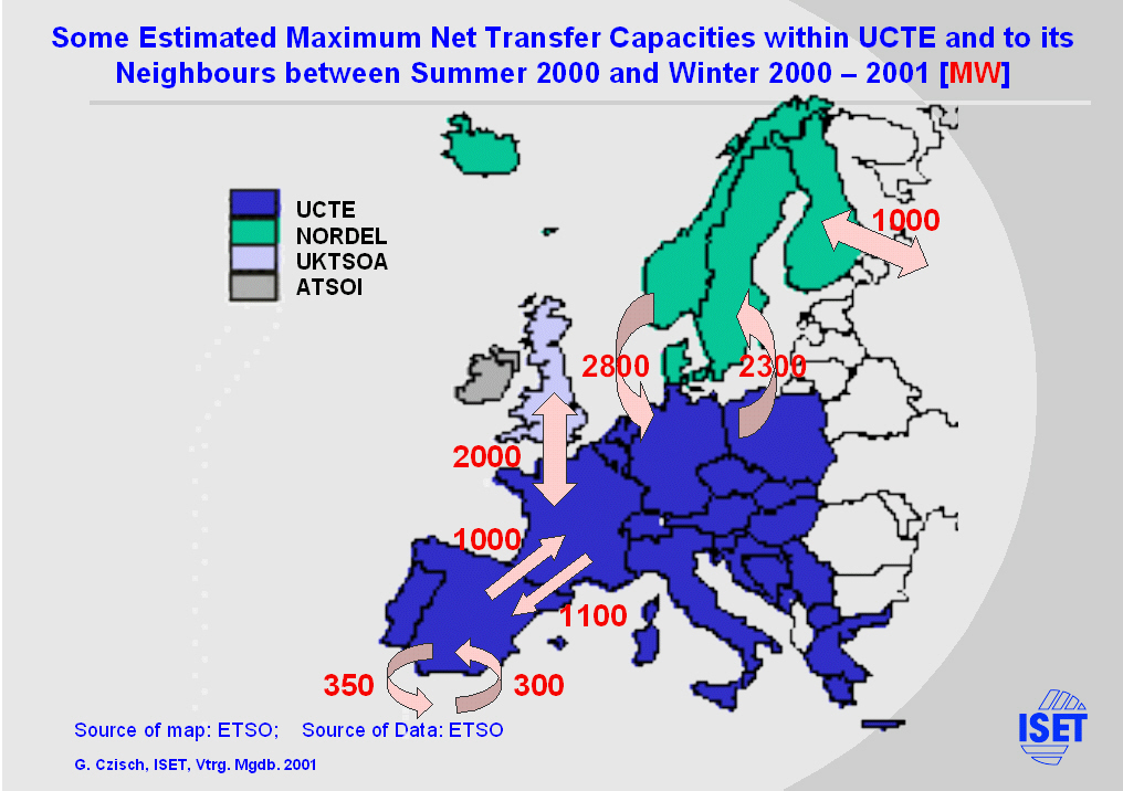
The European electricity network within and especially between the countries is too weak to transport significant amounts of electric power from distant regions with good conditions for renewable electricity production. This is also true for the connection to Africa.
For example the Net Transfer Capacities from Morocco to Spain with its 350 MW and the 1100 MW from Spain to France would not allow high power transfer. But as e.g. can be seen from the calculations presented in the next slide the construction of new transport capacities using today's technologies economically seems to be quite feasible. |
|
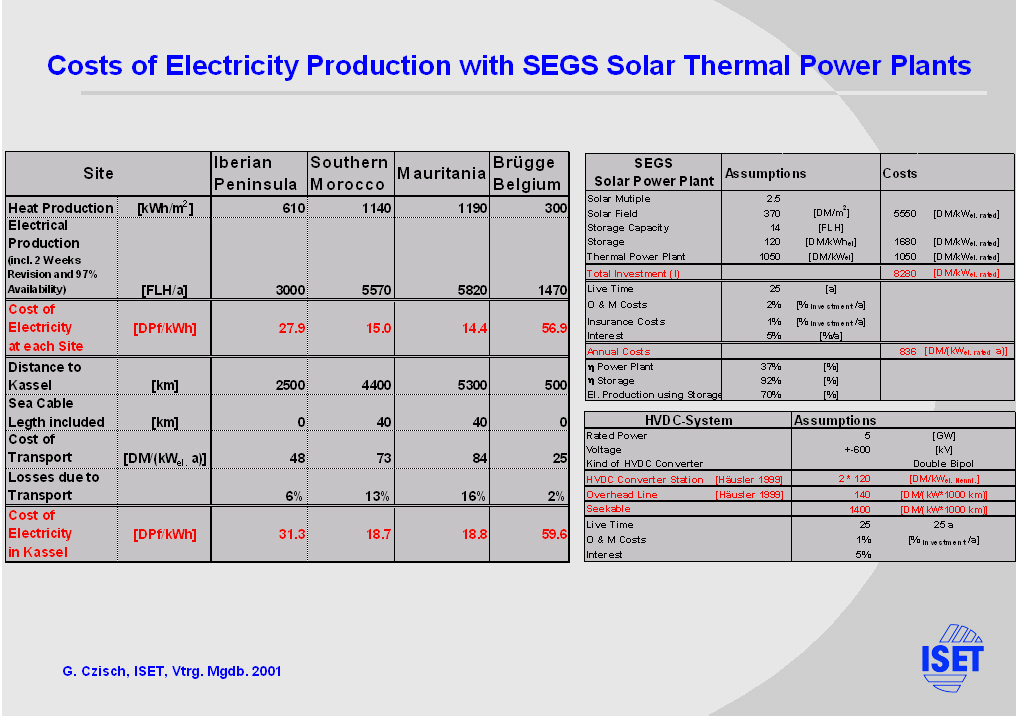
With the underlying economic assumptions based on today's technologies and prices shown in the upper right tables the costs of solar thermal electricity production are calculated for some selected sites. The results are listed in the table on the left side.
Using today's High Voltage DC (HVDC) technology to transport the electricity to Europe (e.g. Kassel GER) the costs of electricity would even for the furthest distance mentioned only increase by 30%. The underlying economical assumptions for HVDC technology are shown in the lower right table. The costs of electricity in Kassel do not seem to be very unreasonable. The option to import solar thermal electricity from Northern Africa to Europe becomes even more interesting if the investment costs for solar fields, the most costly part of SEGS power plants, are reduced. A reduction to roughly 50% of the today's field costs is expected as soon as a capacity of 7 GW of SEGS is erected world-wide. This will reduce the costs of electricity in Kassel to approx. 60% or below 12 DPf/kWh. |
|
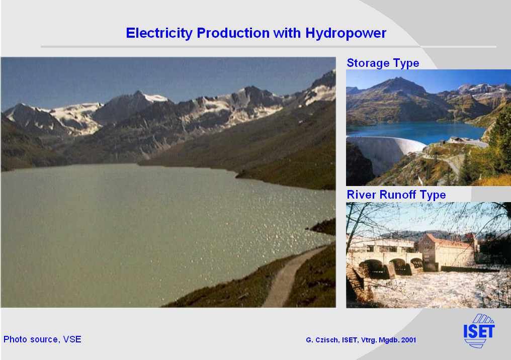
Now we come to hydropower. Here it is interesting to distinguish between two types. The river runoff type uses the water at the time it runs down the river and normally has no or just very little storage capacity. The storage type sometimes can store the water which runs into its reservoir for many months (see following table). So this kind of power plant decouples runoff and electricity production and thus gives the degrees of freedom necessary to be used as back up to balance the variation of other production facilities and of the demand. |

|
This table shows the rated power, the storage capacities and the annual energy production of Storage Hydroelectric Power Plants in Western European Countries. The storage capacities are close to 10% of the total electricity production within all the member countries of the EU. |
|
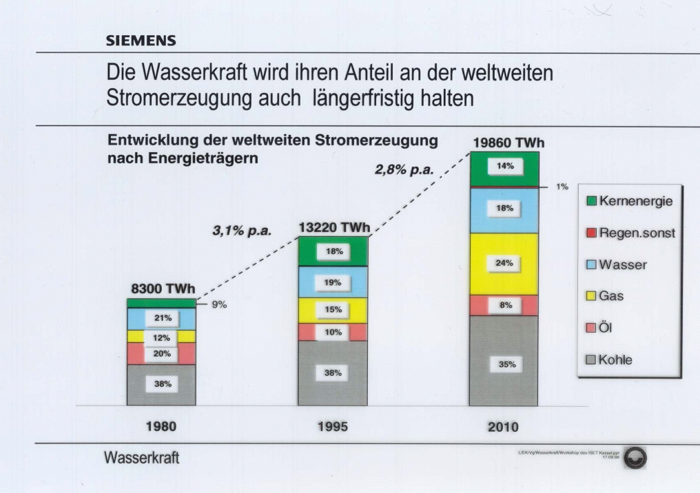
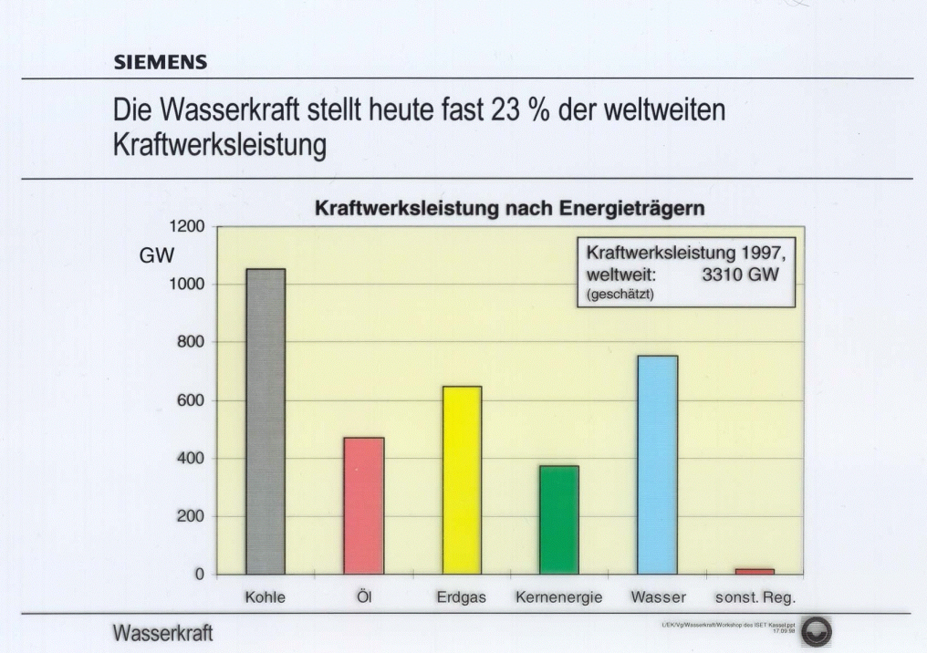
Today 19% of the world wide electricity production is from hydropower. Siemens expects that this fraction will slightly decrease since the estimated growth of the demand with 2.8%/a is higher than the estimated growth of electricity production from hydropower. |
|
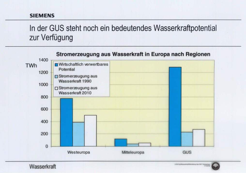
Siemens estimates that within eastern and middle Europe about half of the economically exploitable hydropower potential already is exploited. Within CIS (Commonwealth of Independent States) still very high potentials are available. |
|
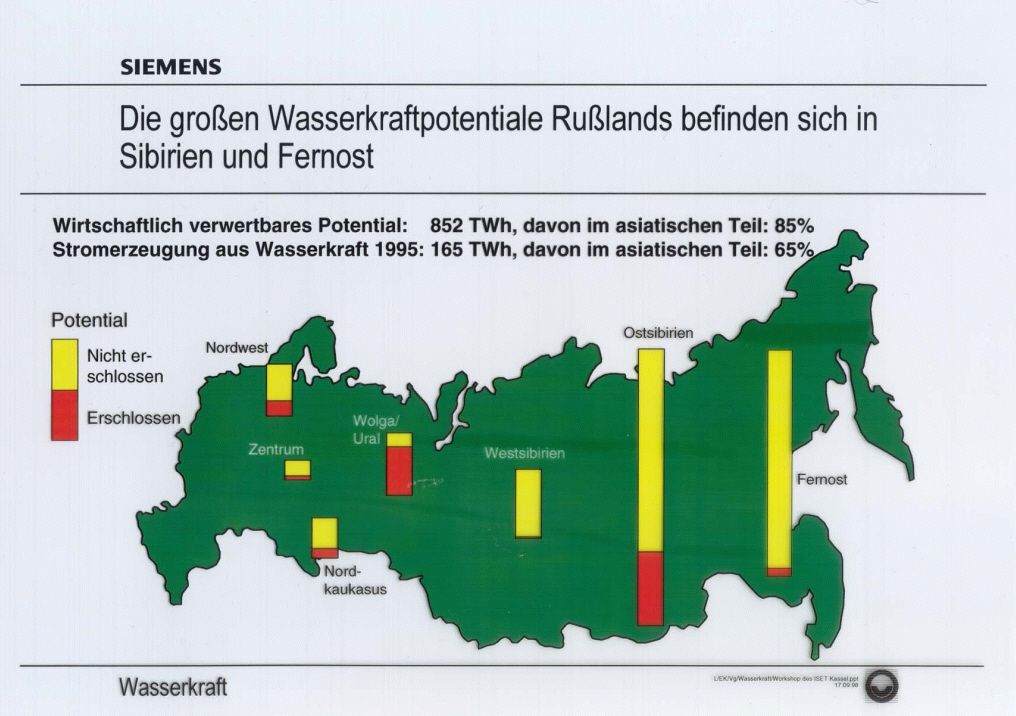
Most of the unused Russian economically exploitable hydropower potentials are in the eastern parts of the country, but even within the European part some remarkable potentials are left. |
|
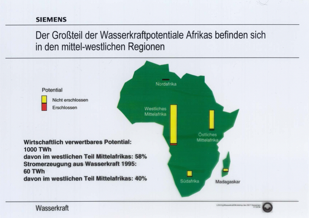
Within Africa the economically exploitable hydropower potentials are also very big. Possibly the best site worldwide for hydropower is close to Inga at the Congo river. Lahmeyer International estimates that the runoff at the best position for the power plant is sufficient to deliver 38 GW of electrical energy more than 355 days per year. The costs for a power plant with some GW Rated power could be approximately at 1000 DM/kW. |
|
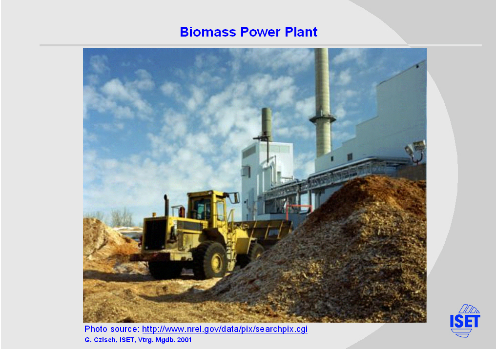
Now we come to electricity production from biomass. |
|
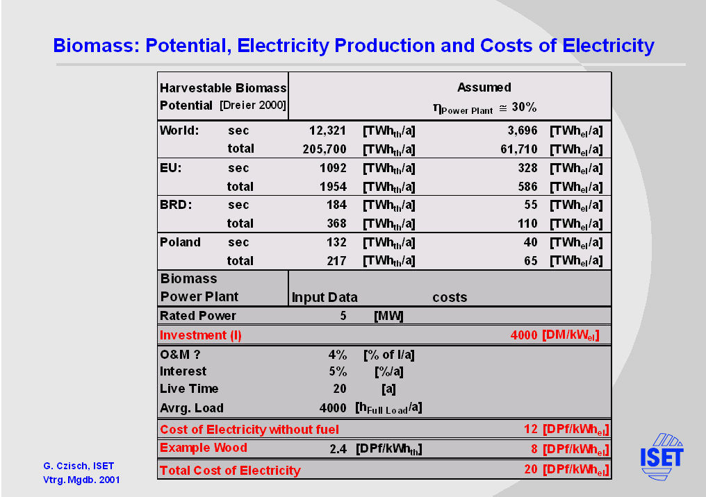
In the upper table biomass potentials estimated by Thomas Dreier ("Lehrstuhl für Energiewirtschaft und Anwendungstechnik, Technische Universität München") are given. The secondary biomass potential is the potential of residues and waste, while the total potential includes the possible biomass production on unused land and within western Europe also 15% of the today's farm land is considered to be usable for this purpose.
Assuming an efficiency of 30% for biomass power plants the secondary resources would be sufficient to e.g. deliver roughly one third of the annual Polish electricity consumption. The lower table exemplary shows a calculation for cost of electricity from Biomass.
|
|
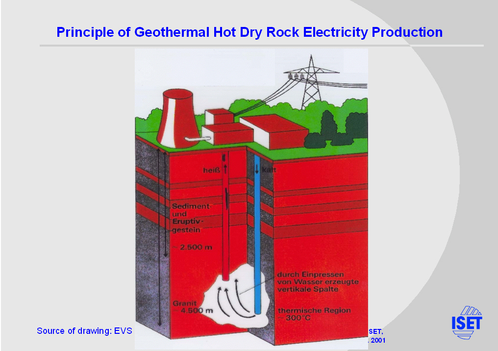
Now we come to geothermal electricity production via Hot Dry Rock technique (HDRt).
The principle of the Hot Dry Rock technique is shown in this slide. At least two wells have to be drilled to a depth of approximately 4000m. One of the wells is used to press water into the porous rock. Here the water heats up and within the second well it flows up to feed a thermal power unit which produces electricity. The HDRt enlarges the geothermal potential since the places where steam or hot water is found which could be used directly to drive a thermal power plant are very rare. |

|
The costs of electricity from geothermal Hot Dry Rock power plants are very dependent on the temperature gradient.
Here the attempt is made to estimate the costs starting from a reference case from the Electric Power Research Institute (EPRI). The assumptions of the reference case and of the underlying economic figures are given in the upper table. Temperature gradients as high as in the reference case will only be found at very few locations on earth, while temperature differences of e.g. 170 K between surface and 4000 m depth are much more common but still far better than average conditions. These conditions would probably allow the production of electricity at costs of 35 DPf/kWh. |

|
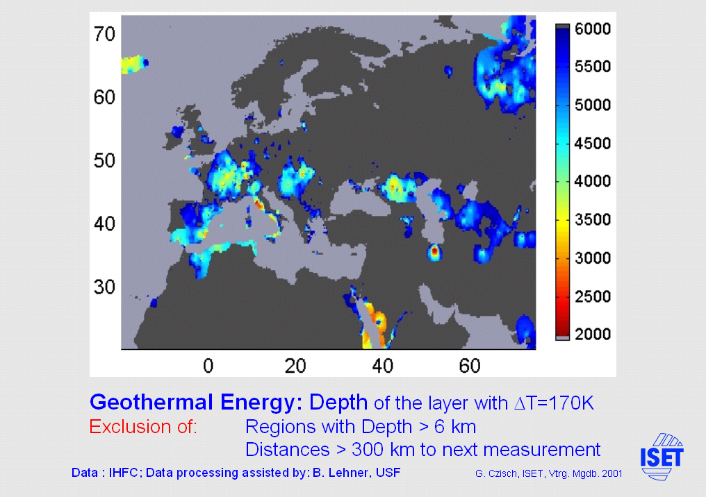
Here we see the depth of the layer at which a temperature difference of 170K to the surface conditions is reached. The grey land regions are regions where the next measurement registered within the data collected by the International Heat Flow Commission (IHFC) is more than 300 km away. The darkest blue indicates regions where the depth of the 170K layer is below 6000m. |
|
Here we see the depth of the layer at which a temperature difference of 170K to the surface conditions is reached. The grey land regions are regions where the next measurement registered within the data collected by the International Heat Flow Commission (IHFC) is more than 300 km away or where the depth of the 170K layer is below 6000m. |
|
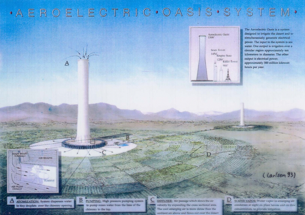
Now we come to a renewable energy system which has not yet been built in an operational size but carefully studied in detail since many years. The conclusion of these studies is that it will be possible to build the necessary towers of more than 1000m height and furthermore, it seems as this could be done at costs that make this kind of electricity production economically very attractive. Moreover the temporal behaviour seems to be quite good compared with other methods that depend on the actual climate conditions. The name used in the following is "Energy Tower". |
|
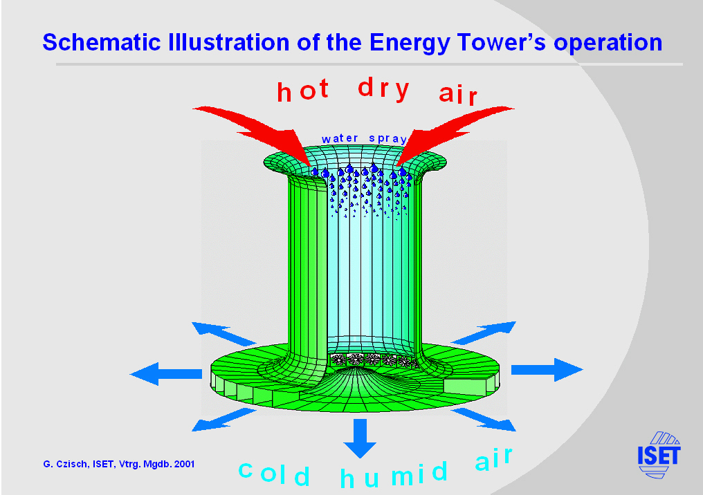
This illustration shows the principle of the Energy Tower. The tower should be sited within a hot and dry climate at relatively short distance (less than 100 km) to big water resources (normally the nearby sea). The water is pumped up to the top of the tower (chimney) and then sprayed into it. There it evaporates and thus cools down the air which as a consequence increases its density. The density difference between outside and inside air is the driving force which causes the downdraft within the chimney. This falling air is used to power turbines to produce electricity. |
|
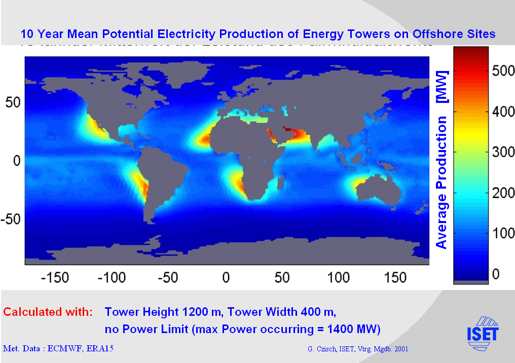
Here the offshore conditions for Energy Towers of a specific design are given as annual average load. The calculations are made using data of the ECMWF and including program code developed by Vadim Mezhibovski (Technion, Haifa, Israel).
The offshore conditions demonstrate very well where the best climate conditions for Energy towers can be found. Here neither transportation nor elevation losses for delivering the water to chimney‘s foot accrue. The best locations are found at the cost lines of the desert belts, where e.g. Passat Winds provide the dry and hot air. |
|
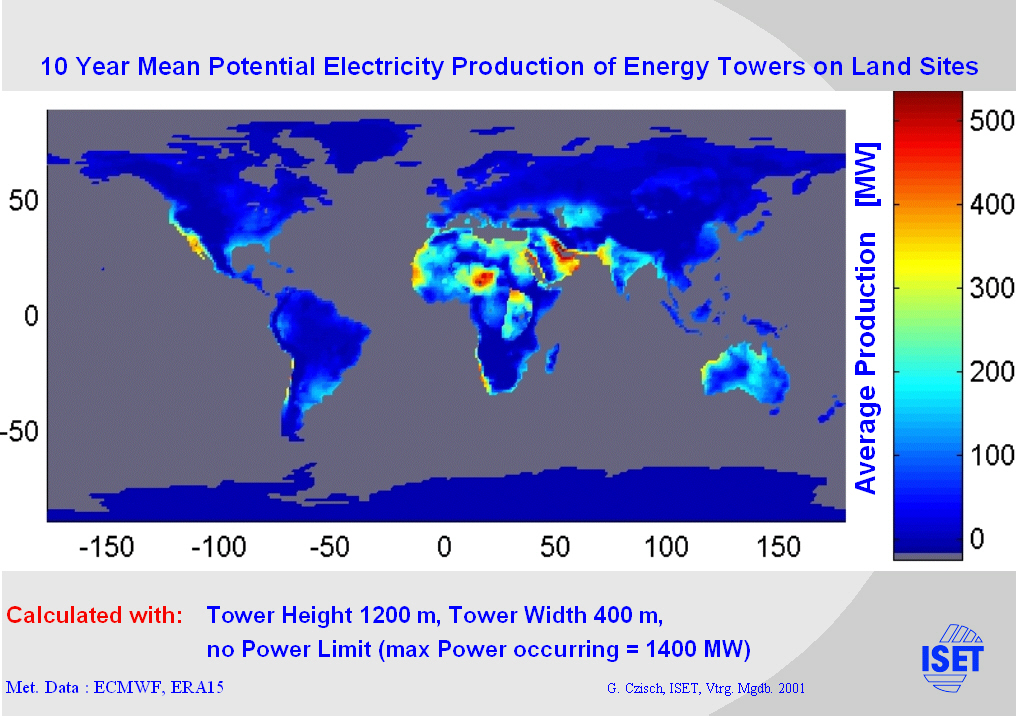
Here the conditions for land based Energy Towers of a specific design are given as annual average load. The calculations are made using data of the ECMWF and including program code developed by Vadim Mezhibovski (Technion, Haifa, Israel).
The conditions on land are strongly influenced by the transportation and elevation losses for delivering the water to the chimney‘s foot.The best locations are found at the cost lines of the desert belts, where e.g. Passat Winds provide sufficient dry and hot air, the distance to the water sources are short and elevation to the towers base is low. From a European point of view the areas in the western Sahara and in the Persian Gulf are most interesting. |
|
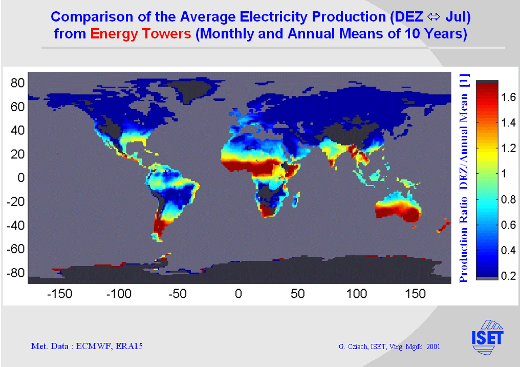
The seasonal variation of power production from Energy Towers is significantly lower at lower latitudes.
On this slide you can see for example the ratio between the average annual electricity production and the production in December. E.g. at the mid Saharan west coast we find that the production only slightly changes over the months. Some hundreds of kilometres south significantly higher production in European winter time can be found. |
|
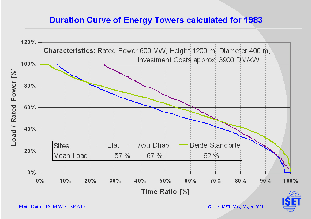
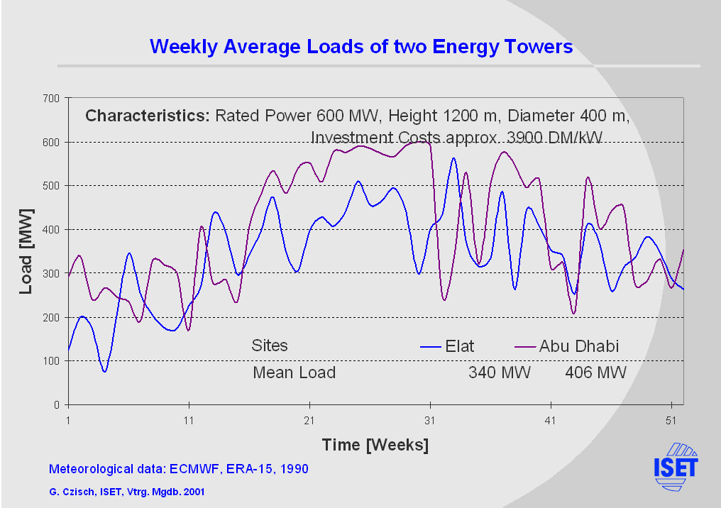
The temporal behaviour of energy towers is very advantageous compared with many other renewable energy systems. Since the dry air is available day and night the daily variations are relatively small.
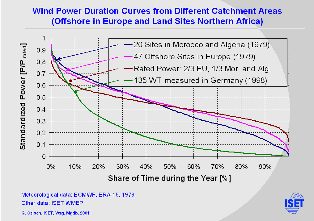
At good sites such as for example in the Persian Gulf region the climate would allow at least a small production at any time during the year. This can be seen from the calculated duration curve of an Energy Tower near Abu Dhabi. At this site the production reaches 40% of the rated power within 78% of the time during the year. A combined production of two Energy Towers, e.g. one close to Elat and the other about 1300 km away in Abu Dhabi, shows that the combination could further improve the temporal behaviour. |
|
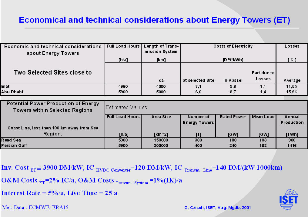
With the underlying economic assumptions based on today's technologies and prices for High Voltage DC (HVDC) transmission systems and based on estimations for the Energy Towers - both shown below the tables - the costs of electricity are calculated for two selected sites. The upper table shows the results for the local costs as well as for the transmitted electricity in Middle Europe (Kassel).
The costs of electricity in Kassel economically seem to be very interesting and thus would justify further research and efforts to erect at least a small scale pilot plant. |

|
Now we come to wind energy which today may be the most attractive and promising form of renewable energy use.
At the moment the highest rated power of Wind Turbines (WT) available in the market is 2.5 MW, while some efforts are being made to develop WTs with a rated power up to 5 MW. |
|
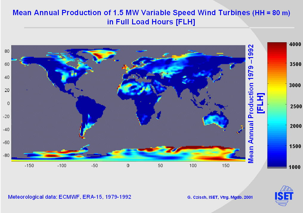
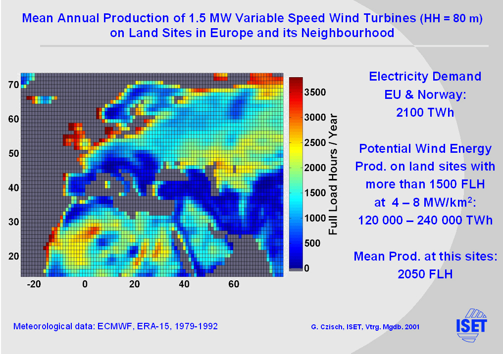
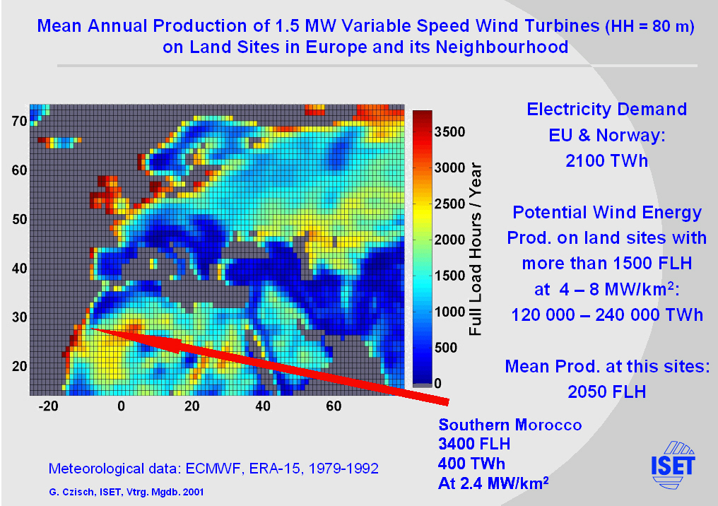
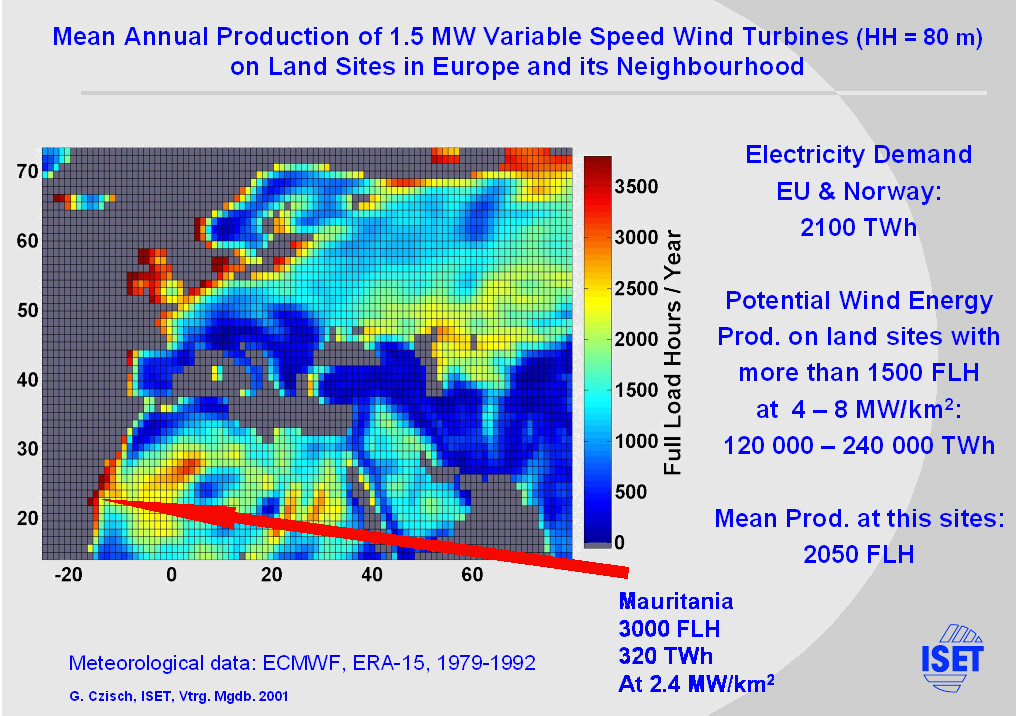
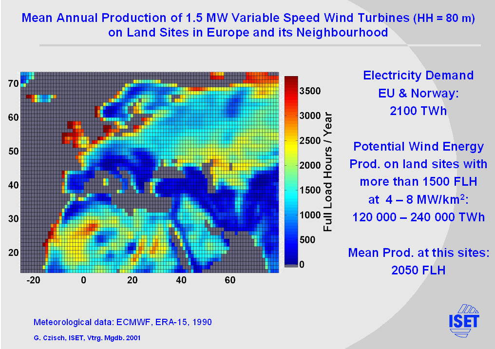
Here we see the potential production of wind energy calculated from data of the European Centre for Medium Range Weather Forecast (ECMWF) expressed in FLH. Europe itself has good wind conditions. But its use is limited by the high population density. In a belt 4000 to 5000 km away from Kassel (Germany) there are also very good wind conditions and in most of the areas the population density is 2 orders of magnitude smaller than for example in Germany. |
|
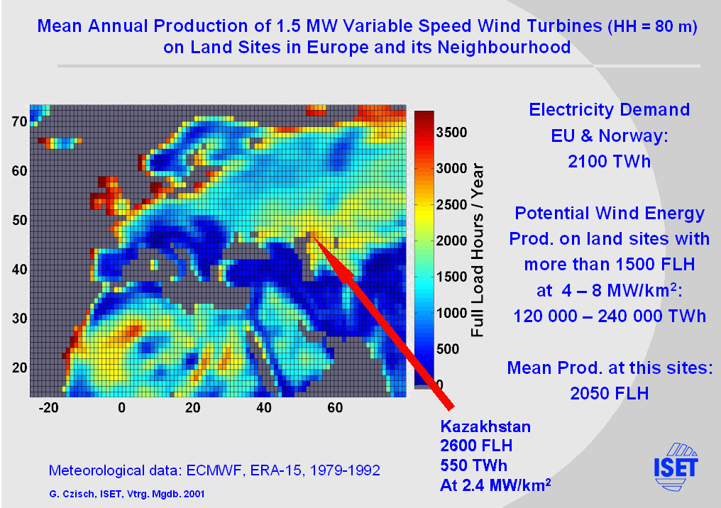
If we now zoom in and look at Europe and its neighbourhood we find that the potential production within the shown area only considering sites with a potential annual production of more than 1500 FLH is about 100 times higher than the need of the European Union and Norway together. |
|
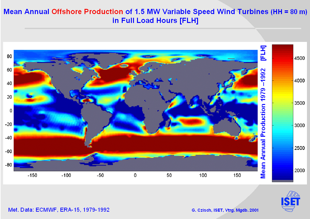
Here we see the potential offshore production from wind energy calculated with data of the European Centre for Medium Range Weather Forecast (ECMWF) expressed in FLH. Europe itself has good wind conditions as well in the North Sea as in the Baltic Sea. |
|
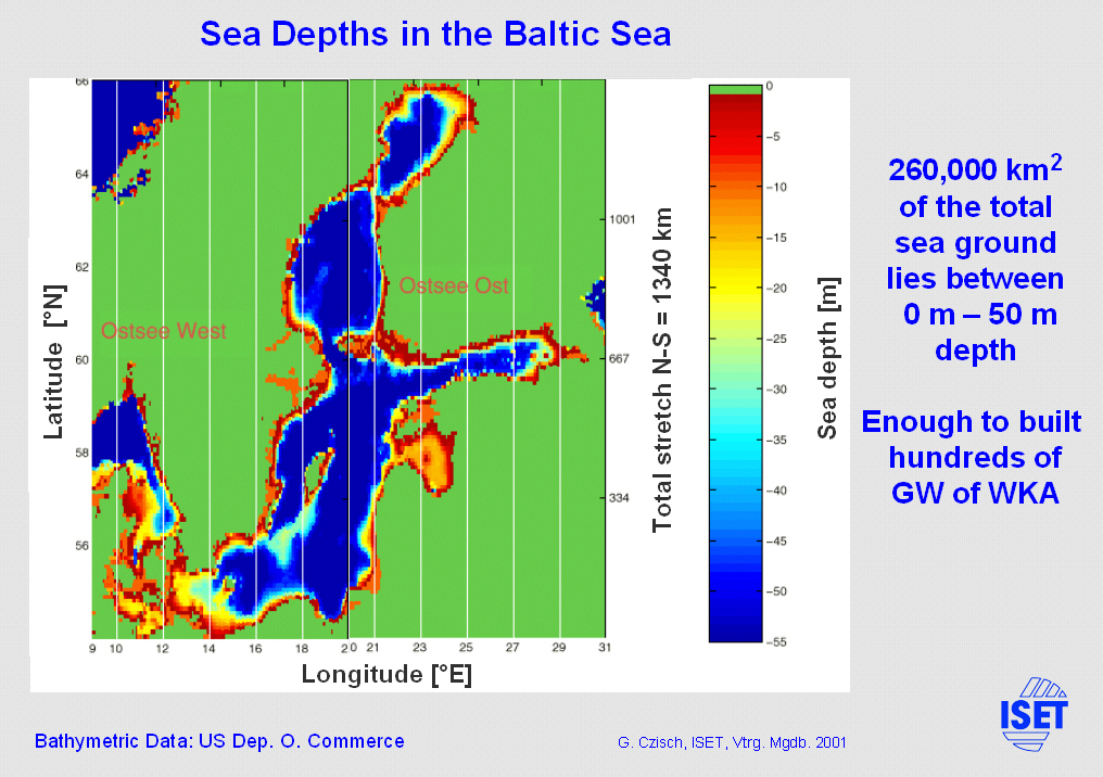
The use of offshore wind energy is dependent on relatively low depths of the sea ground. Today some offshore wind farms are planned within areas with up to 40 m depth. So it seems to be reasonable to select areas where the depth lies within this order. On this map the depth up to 55 m are displayed for the Baltic Sea. The total area flatter than 50 m is 260000 km^2. At 4 MW/km^2 this would be sufficient for 1000 GW of erected wind turbines and thus allows a careful selection of the best sites where negative environmental and other unfavourable effects can be minimized and the sites with better wind conditions could be chosen. |

|
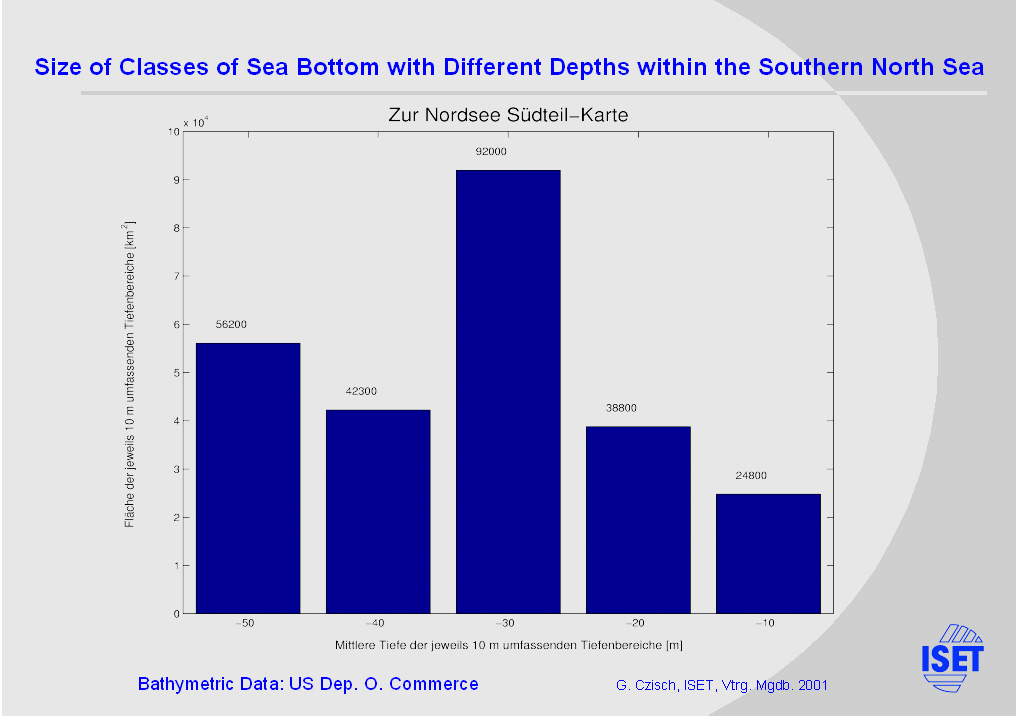
On this map depths up to 55 m are displayed for the North Sea. |
|
The total area flatter than 55 m is 250000 km^2. At 4 MW/km^2 this area would be sufficient for 1000 GW of erected wind turbines and thus allows to carefully select the best sites where negative environmental and other bad effects can be minimized and the sites with better wind conditions could be chosen. |
|
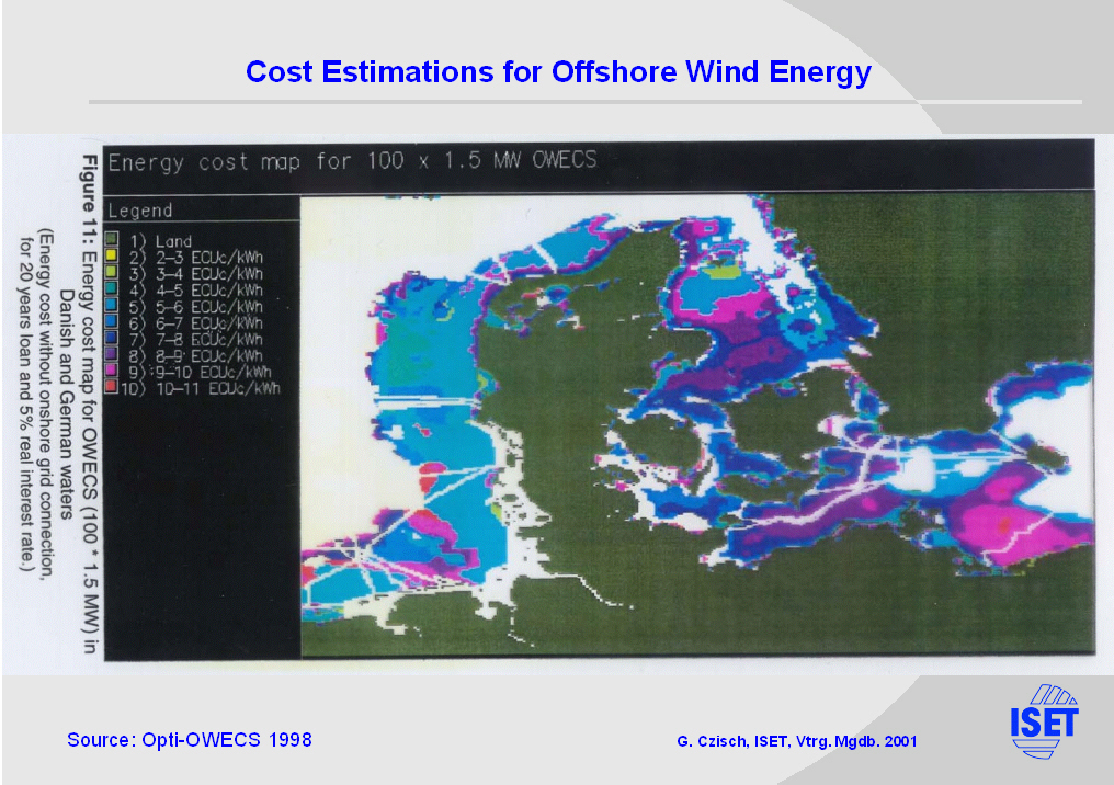
On this map cost calculations for offshore wind parks of 150 MW rated power with wind turbines each 1.5 MW are displayed. At the best sites where the wind conditions are good, the seafloor is not too deep and also other conditions are advantageous, the costs of electricity are estimated to be within the range of 3 to 4 €c/kWh. |

|
The seasonal variation of the potential power production from wind energy shows significant varieties in different regions.
On this slide you can see for example the ratio between the average electricity production in July and January. We see, that Europe is a typical winter wind region with maxima in winter and minima in summer. While for example at the Saharan west coast we find maxima of the production in summer. In some other regions the production in July and January are quite similar. So the idea of selecting the regions in order to get the best match of production and electricity consumption suggests itself. |
|
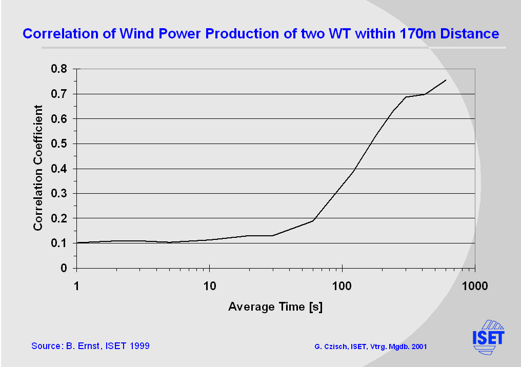
This diagram points out the spacio- temporal behaviour of wind power.
Here you see the correlation of the change of power from two wind turbines printed versus the averaging time. It can be derived that fluctuations due to the low correlation within shorter time intervals of some minutes can be smoothened even within one bigger wind park. |
|
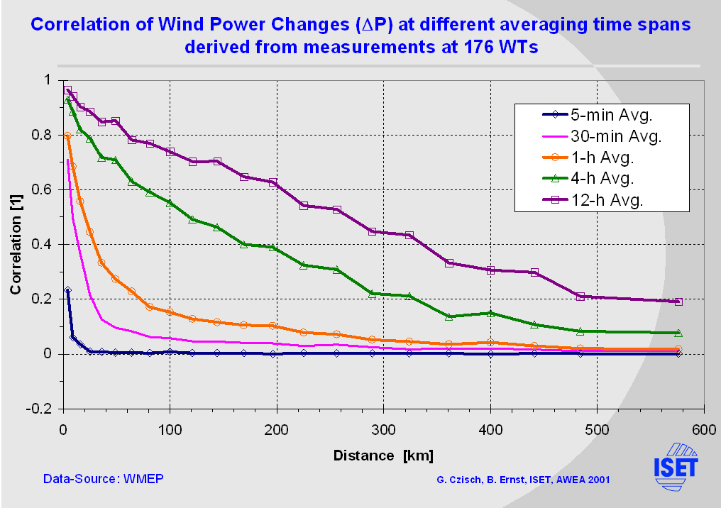
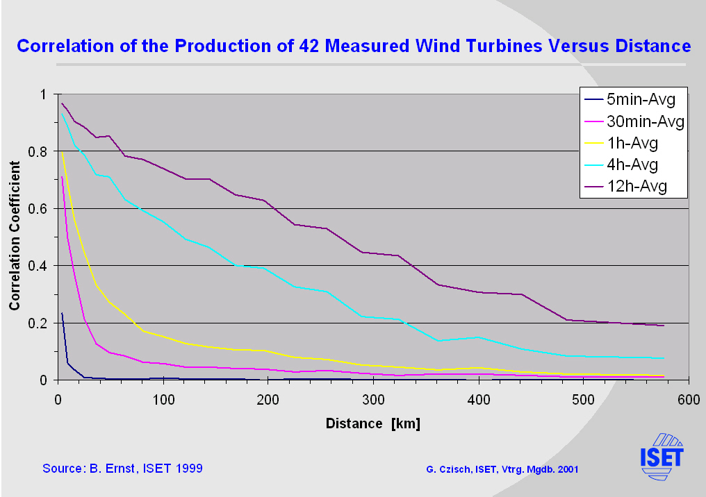
This graph shows the correlation of the change of wind power printed versus the distance between the wind turbines. This is given for different averaging times.
For example the 5 minute correlation falls to almost zero after a distance as short as 20 km. While the 12 hour values reach a correlation coefficient of 0.2 at a distance of 500 km. |

|
Till now we only have studied measurements within Germany. Further on we are going to look at Europe and its neighbourhood shown in this map.
By the way: The potential production within the area shown only considering sites with more than 1500 FLH is about 100 times higher than the need of the European Union and Norway. So it is possible to be quite selective and choose only the better regions. |
|
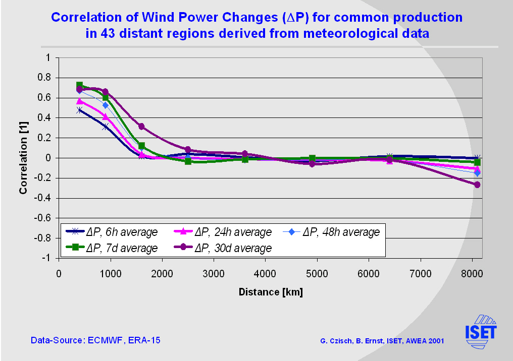
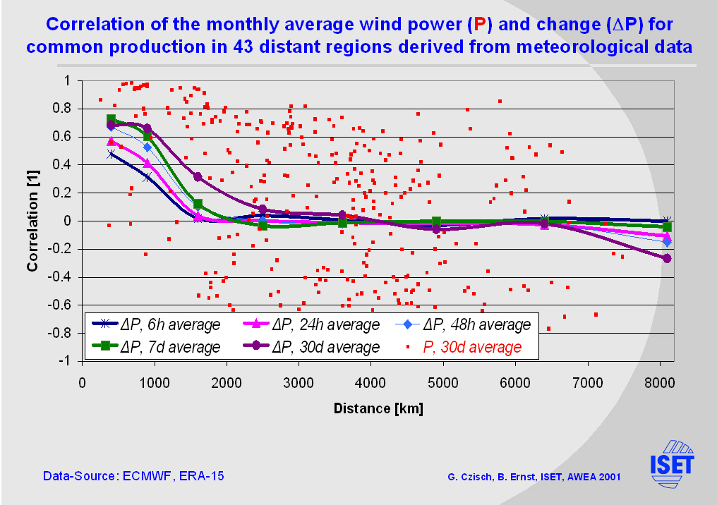
From the region shown on the previous slide 43 subregions with good wind conditions have been selected to study the temporal behaviour of their potential wind power production. Here the mean correlation of the power changes is shown over the region‘s distance.
As we see from the monthly mean, which is the violet line, the mean correlation drops down to almost zero at a distance of roughly 2000 km. This means that even considerable monthly smoothing effects can be achieved as soon as the catchment area reaches this sizes. |
|
If we look in detail at the correlation of the monthly mean wind power itself, we see that regions can be found where the production is quite well anticorrelated to others. Some of this anticorrelations are of systematic nature. So the idea of selecting the regions in order to get the best match of production and electricity consumption suggests itself. |
|
|
|
|

|
As mentioned before the potential production within the area shown only considering sites with more than 1500 FLH is about 100 times higher than the demand of the European Union and Norway. So it is possible to be quite selective and choose only the better regions. As an example I selected the following.
To use these potentials we have to have high transport capacities. |
|
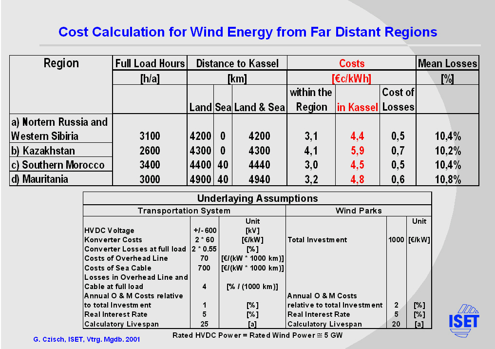
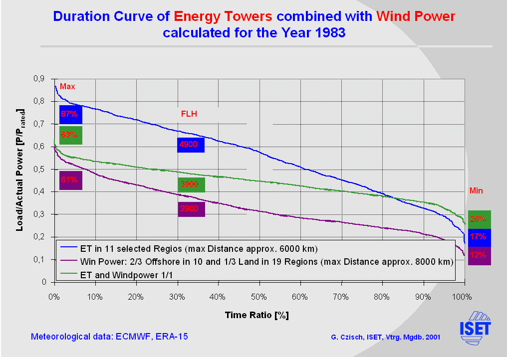
Economically the option of wind power import is interesting even when new transport capacity is included.
But not only the low population density and the low costs of imported wind power are notable. The temporal behaviour of the power production changes with the size of the catchment area and with the different kinds of climate conditions. |
|
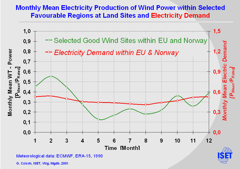
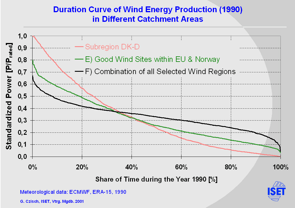
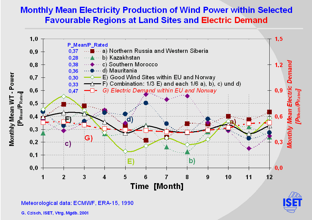
Comparing the monthly mean wind power of the selected European regions and the demand of the EU & Norway one can see that the fluctuations of the production vary much more than the demand. Europe is a typical winter wind region with maxima in winter and minima in the summer months. |

|
The monthly means in Southern Morocco also vary much more than the demand, but it is a passat wind region with summer maxima. |

|
It is obvious that the use of simultaneous production in different regions can match the demand much better.
This shows the black line which represents a combination of the five selected regions. But not only the long term behaviour changes with the size and selection of the catchment area. |
|
|
|
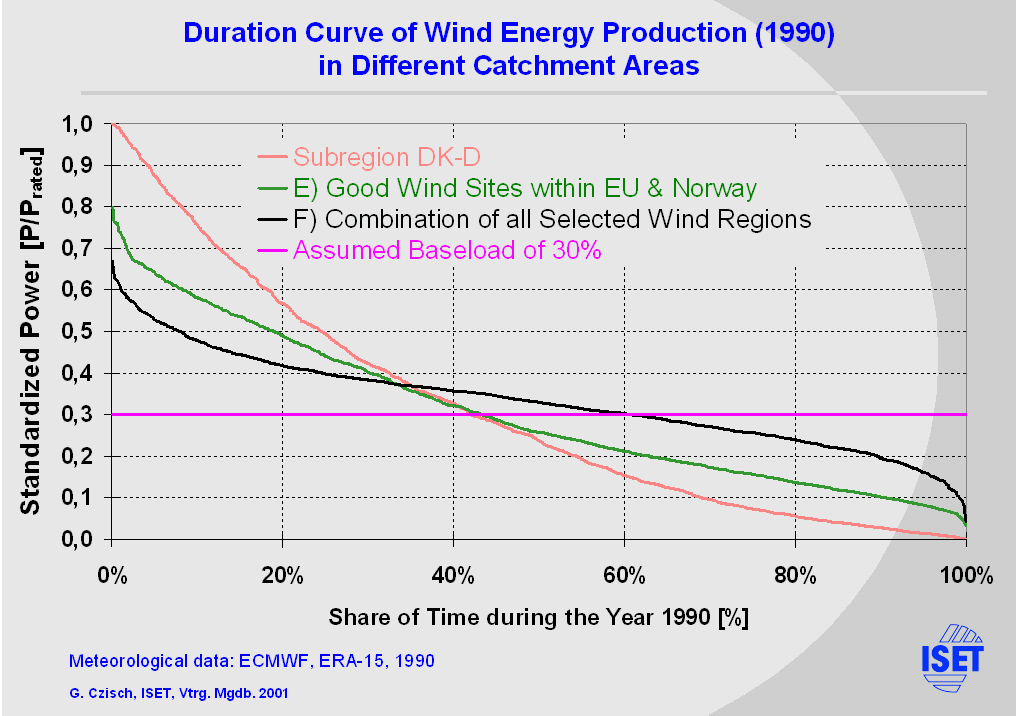
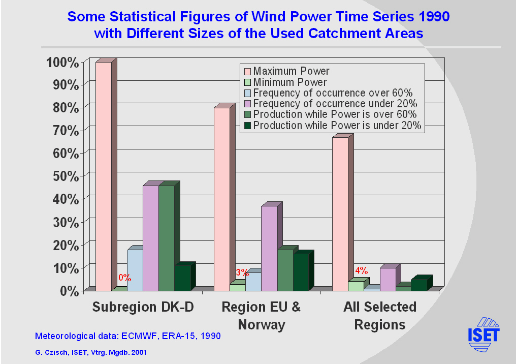
Let us assume we want to produce a base load of 30%. Now we have some excess and some lack of power. |

|
For example the smallest region would produce 40% of the base load in excess but on the other hand there would be 36% missing.
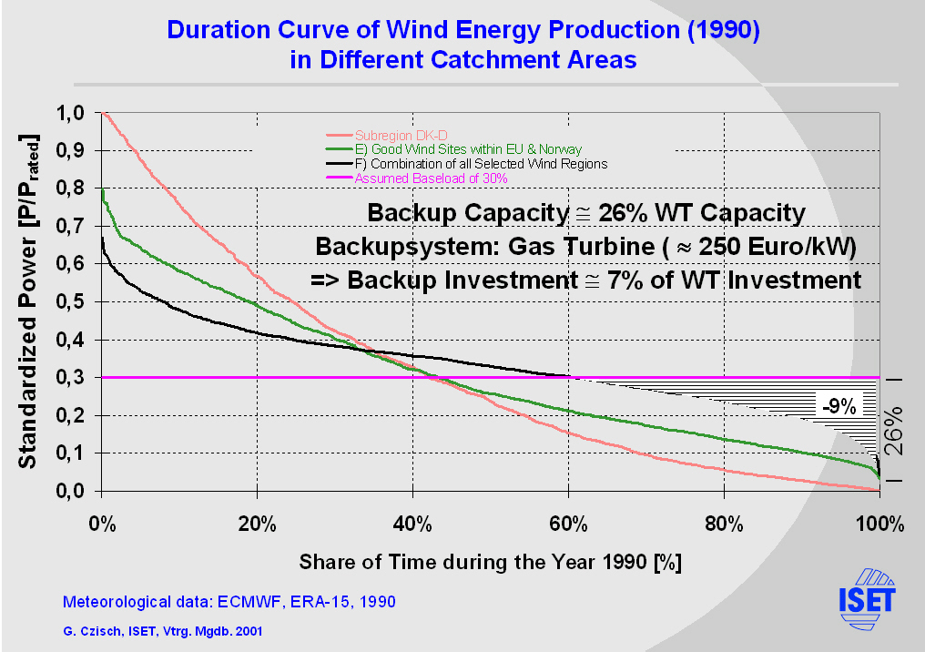
With simultaneous use this lack declines to only 9%. |
|
So we would need this 9% as backup energy and a rated backup power of 26% of the wind turbine capacity.
This could be produced from gas turbines, which cost roughly 250 €/kW. (In the last years the market for gas turbines has grown considerably and therefore, the prices almost doubled to 500 €/kW in 2001.) The investment in the backup system is about 7% of the investment in the wind turbines. If we now consider producing the equivalent of the demand from wind Energy. For the demand EU & Norway we need to install 660 GW to within all regions. |
|
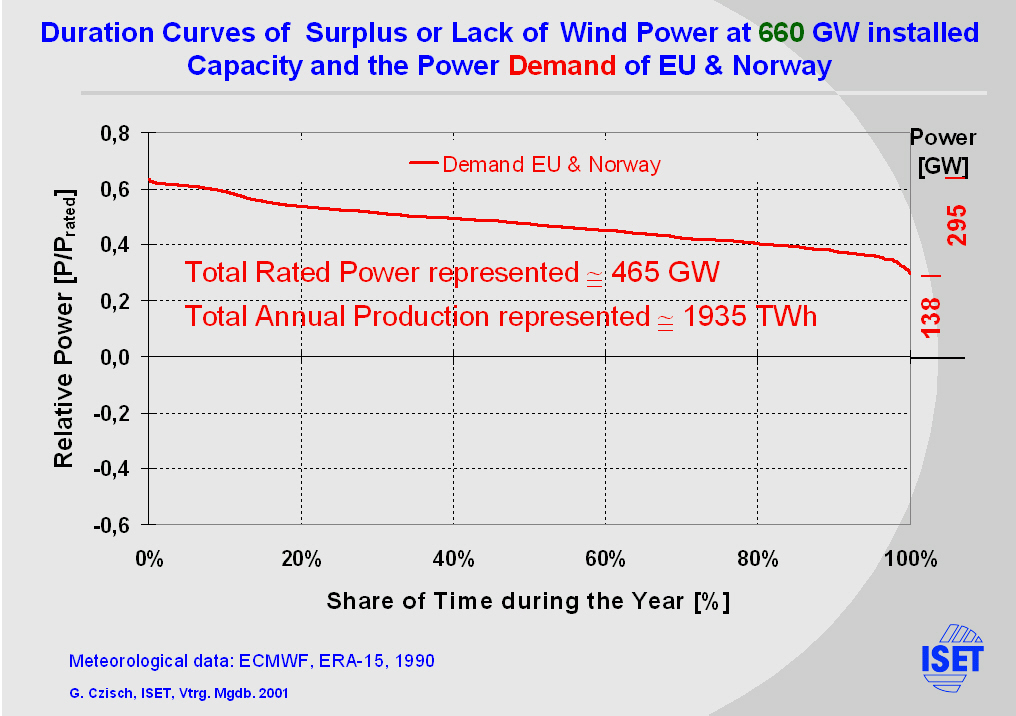
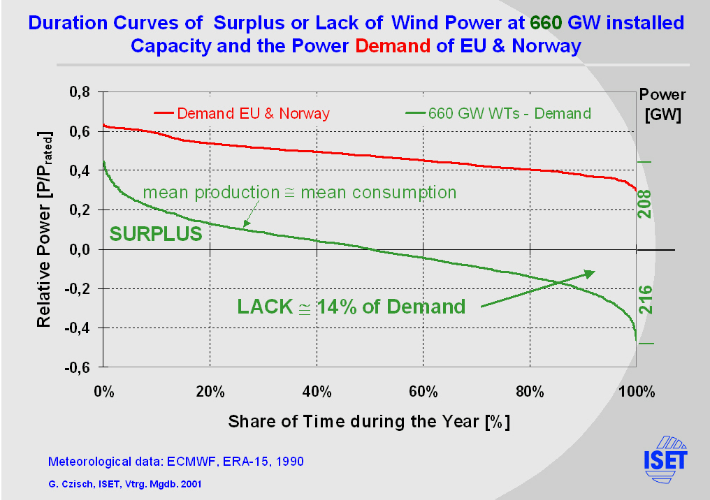
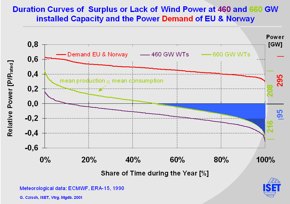
The duration curve printed in the slide represents a total rated power of 465 GW and a demand of 1940 TWh.
The maximum power demand is 295 GW, the minimum about 140 GW. |
|
The difference between wind power production and demand is shown in the green line. The maximum power surplus and lack are each roughly 200 GW. The lack of energy amounts to 14% of the demand. |
|
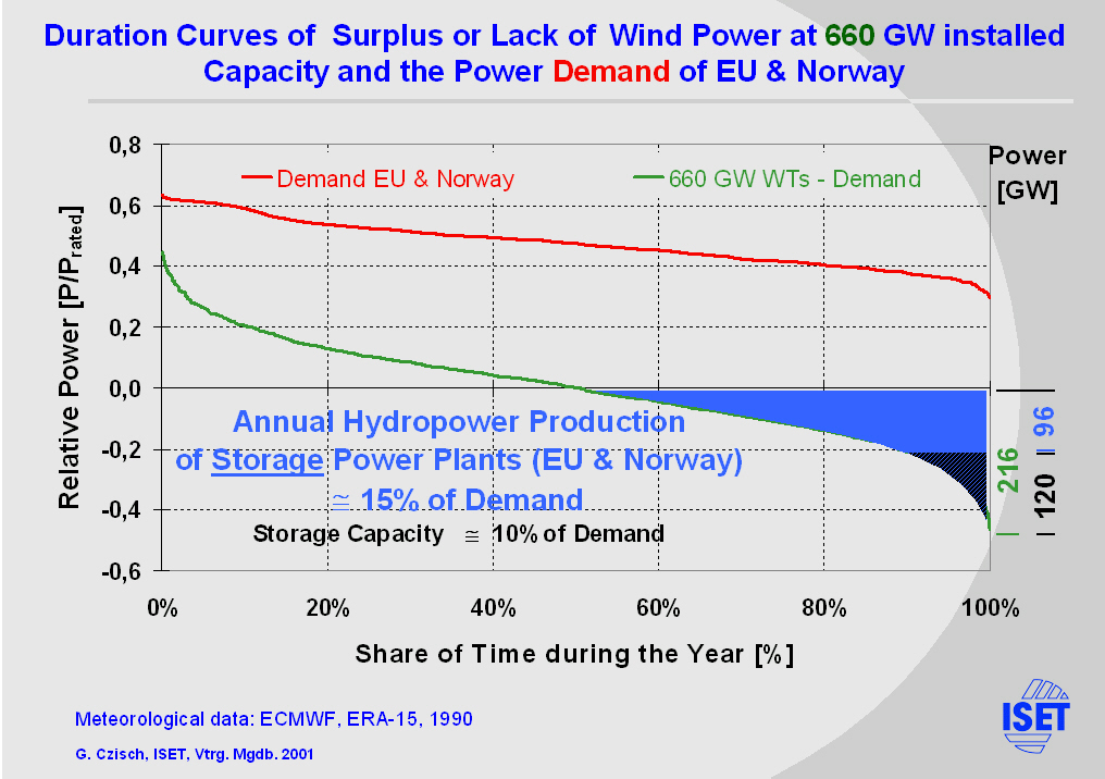
In Europe storage systems exist with relatively high rated power and storage capacities.
The annual production of the storage hydropower within our supply area is 15% of its demand. So it is slightly higher than the lack of energy from the considered wind power production and so more than enough to compensate the lack of energy. But the 96 GW rated power of the storage hydropower plants is too small to compensate the lack of power. The difference is still 120 GW. There are many possibilities to get the necessary backup power. One is to enlarge the rated power at the reservoirs as it sometimes is done to provide peak load capacity. Another way is to use thermal units which could also could be fired by Biomass. |

|
At the end of my talk I want to switch the point of view to an other aspect of the Extraeuropean option for an energy supply with wind power. I roughly want to sketch the idea to combine CO2 reduction and Development aid. Therefore I will compare to potential partners within a new electricity system.
Morocco and Germany: The population of the developing country is about 36% of the German population. In Morocco the electric consumption per capita is 7% of the consumption in Germany. The GDP is just 1.7% of ours. It really is a poor country. In Germany we spend 2.2 % of our GDP on electricity, which is more than the total Moroccan GDP. If the EU decided to produce 10% of its electricity in Morocco (equivalent to 40% of Germany's consumption), the total investment in wind parks is on the one side only 3.3% of Germany's annual GDP or 1 ½ times our annual expenditures for electricity. On the other side it is 2 times the actual GDP of Morocco. So the decision for us would mean to get relatively cheap electricity and for Morocco it could provide development aid that would last for some decades. |
| ANNEX | |
|
|
|
|
|
|
|
|
|
|

|
|
|
|
|
|
|
|
|
|
|
|
|
|